

NoteReviewers
- Ryan Peterson (2025-11-24).
- Patrick Breheny (2025-12-12).
What connotation do you attach to the word “bias”? A negative one?
In this post we will see why not all bias is bad… at least when it comes to building predictive models. In fact, for many years, statisticians have recognized the benefits of biased estimators in reducing prediction error. Perhaps you knew this, but if not, don’t worry. That is the purpose of this post.
$$
% Uppercase roman letters
% Lowercase roman letters (c, d, u, v have to be treated special; see end)
%% Roman letters with hats
%% Roman letters with subscripts
%% Roman letters with tildes
%% Script letters
%% Greek letters
%% Greek letters with tildes
%% Operators
%% Statistical
% Fisher/observed information% Independence
%% Mathematical %% %% Requires dsfonts
%% Equations
% Other
$$
Modeling Goal
When starting off with a data analysis, it is important to outline the primary goals. Whether you realize it or not, in virtually all cases, a primary goal is to use the data to develop a predictive model.
Consider a clinical trial evaluating a new drug for metastatic lung cancer. We say our goal is to “estimate the treatment effect” of our new drug. However, estimating a treatment effect is fundamentally a predictive task. That is, we need to predict what would happen with treatment and what would happen without treatment. The treatment effect is the difference between those two predictions*, the better our predictions… the better our estimate of the treatment effect is.
NoteA pre-dictor is pre-what, exactly?*
When we say a treatment effect is “the difference between two predictions,” that only works if the predictions are made using information that comes before the treatment starts. These are true pre-treatment predictors.
If we accidentally include a model “predictor” that is measured after treatment begins, the treatment could affect it, and the real treatment effect gets obfuscated. The model might appear to “predict” well, but the truth is that it’s not “predicting” at all. Models built this way can give a misleading estimate of the effect of the treatment because part of the effect has been absorbed by the post-treatment variable.
For a valid treatment effect, we must base predictions only on information that could not have been influenced by the treatment – valid pre-dictor variables.
Now, suppose with treatment alone we can predict remission status with 60% accuracy. If you also have patients’ genetic information, what should you do with that?
Including it directly into a model is problematic because the human genome is large*. Unless you have a massive number of patients in your trial (hundreds of thousands) you will NEED to make assumptions about the plausible effects of someone’s genetic information on how well the new treatment works. These assumptions allow us to fit a model with all the genetic information but also intentionally introduce bias to the estimates. This is what a method known as penalized regression does, which we will cover momentarily.
NoteHuman Genome*
The human genome is estimated to contain between 30,000 and 40,000 genes!
Now, suppose including genetic information allows us to predict if a patient will be experience remission with 75% accuracy. But this was with biased estimates?! Surely, if we could remove this bias we would get even better predictions, right?
To answer this, we will now break down what makes a set of estimates good at prediction.
Breaking down predictive performance
NoteBias-variance tradeoff
When we estimate parameters for a model, we are always juggling two competing forces: bias, which measures how far our average estimate is from the truth and variance, which reflects how much our estimates would change if we collect a new sample. A model’s ability to predict an outcome is dependent on both. Increasing or inducing bias can often reduce variance, whereas decreasing bias can often increase variance. Good predictions come from striking a balance between the two. It is not uncommon to be able to intentionally introduce a little bias and be able to drastically reduce variance resulting in better predictive abilities.
It is like comparing one friend who is always 5 minutes late to one that is sometimes 30 minutes early and other times 30 minutes late. While the latter is on average on time, you’d probably describe the one who is always 5 minutes late as more reliable.
If you are someone who likes mathematical details, keep reading. But if the previous example makes sense, feel free to skip to the next section.
For a sample of size \(n\), suppose we have a continuous outcome stored in a length \(n\) vector \(\mathbf{y}\) and \(p\) features on each sample unit stored in an \(n \times p\) matrix \(\mathbf{X}\). We will focus on a linear predictor setting. That is, we want to predict \(\mathbf{y}\) based on a linear combination of the features in \(\mathbf{X}\). We do this by estimating \(p\) parameters \(\boldsymbol{\beta}\) and then obtaining predictions \(\hat{\mathbf{y}}\):
\[ \hat{\mathbf{y}} = \mathbf{X}\widehat{\boldsymbol{\beta}} \]
\(\widehat{\boldsymbol{\beta}}\) is usually estimated in a way that is based on minimizing \(\lVert\mathbf{y}- \hat{\mathbf{y}}\rVert_2^2\), known as the residual sum of squares. However, to assess predictive performance we might consider mean square prediction error (MSPE). MSPE shifts our focus to how well our model is expected to predict a single out-of-sample observation (an observation \(y_0\) with predictors \(\mathbf{x}_0\) that was not in the original sample used to estimate the model).
\[ \text{MSPE} = E \left[\lVert y_0 - \mathbf{x}_0^{\scriptscriptstyle\top}\widehat{\boldsymbol{\beta}}\rVert_2^2\right] = E \left[ (y_0 - \hat y_0)^2\right] \]
Assuming that the error structure for \(\mathbf{y}\) is normally distributed (i.e. \(\mathbf{y}= \mathbf{X}\boldsymbol{\beta}+ \epsilon, \epsilon\overset{\text{iid}}{\sim}\textrm{N}(0, \sigma^2)\)) and letting \(\epsilon_0\) be the error corresponding to \(y_0\) and \(\mathbf{x}_0\), MSPE can be decomposed as follows:
\[ \begin{aligned} (y_0 - \hat{y}_0)^2 &= (\mathbf{x}_0^T \boldsymbol{\beta}- \mathbf{x}_0^T \widehat{\boldsymbol{\beta}}+ \epsilon_0)^2 \\ &= (\mathbf{x}_0^{\scriptscriptstyle\top}(\widehat{\boldsymbol{\beta}}- \boldsymbol{\beta}))^2 + 2 \mathbf{x}_0 ^{\scriptscriptstyle\top}(\widehat{\boldsymbol{\beta}}- \boldsymbol{\beta})\epsilon_0 + \epsilon_0^2 \\ \Rightarrow \text{MSPE} &= E\left[\mathbf{x}_0^{\scriptscriptstyle\top}(\widehat{\boldsymbol{\beta}}- \boldsymbol{\beta})(\widehat{\boldsymbol{\beta}}- \boldsymbol{\beta})^{\scriptscriptstyle\top}\mathbf{x}_0\right] + \sigma^2 \\ &= \mathbf{x}_0^{\scriptscriptstyle\top}E\left[(\widehat{\boldsymbol{\beta}}- \boldsymbol{\beta})(\widehat{\boldsymbol{\beta}}- \boldsymbol{\beta})^{\scriptscriptstyle\top}\right]\mathbf{x}_0 + \sigma^2 \\ &= \mathbf{x}_0^{\scriptscriptstyle\top}\left[\text{Var}(\widehat{\boldsymbol{\beta}}) + \text{Bias}(\widehat{\boldsymbol{\beta}})\text{Bias}(\widehat{\boldsymbol{\beta}})^{\scriptscriptstyle\top}\right]\mathbf{x}_0 + \sigma^2 \end{aligned} \]
To make the point easier to see, assume we have just a single predictor \(x_0\) (i.e., \(p = 1\)) and consider two different candidate estimators for \(\beta\), \(\hat{\beta}^A\) and \(\hat{\beta}^B\). Then, the difference in their MSPEs is:
\[ \text{MSPE}(\widehat{\beta}^A) - \text{MSPE}(\widehat{\beta}^B) \]
\[ \begin{aligned} & = x_0^2 \left(\text{Var}(\widehat{\beta}^A) + \text{Bias}(\widehat{\beta}^A)^2\right)+ \sigma^2 - \left[ x_0^2 \left( \text{Var}(\widehat{\beta}^B) + \text{Bias}(\widehat{\beta}^B)^2\right) + \sigma^2 \right] \\ & \propto (\text{Var}(\widehat{\beta}^A)-\text{Var}(\widehat{\beta}^B)) + (\text{Bias}(\widehat{\beta}^A)^2 - \text{Bias}(\widehat{\beta}^B)^2). \end{aligned} \]
So now we see the details of the earlier claim that predictive performance is a function of both variance and bias of the estimates.
Let’s work through a toy example. Consider an example where estimator A has a bias of -0.5 and has a variance of 1. This scenario might reflect a penalized estimate for \(\beta ^A\), where the estimator wants to shrink the estimate by a certain amount. Consider an alternative estimator B which corrects the bias of estimator A so that \(\text{Bias}(\widehat{\beta}^B) = 0\), but this increases its variance to 1.5. Then
\[ \begin{aligned} (\text{Var}(\widehat{\beta}^A)-\text{Var}(\widehat{\beta}^B)) + (\text{Bias}(\widehat{\beta}^A)^2 - \text{Bias}(\widehat{\beta}^B)^2) &= (1 - 1.5) + ((-0.5)^2 - 0^2) \\ &= -0.25 \end{aligned} \]
The MSPE for the “debiased” estimator is greater than that of the “biased” estimator. Correcting the bias in the estimator had a negative impact on predictive performance.
So, if we care about predictive performance, then bias in our estimates is not necessarily a bad thing.
Penalized Regression
A common rule of thumb is that you need at least 10 observations (\(n\) denotes number of observations) per predictor (\(p\) denotes number of predictors) in traditional linear regression settings to estimate \(\boldsymbol{\beta}\) “stably” using ordinary least squares (OLS), but even more may be required. If \(n > p\) but \(n < 10p\), this rule of thumb would suggest we are in a gray area where estimates for \(\boldsymbol{\beta}\) tend to be highly variable and can lead to poor predictions. Of course, if \(n < p\), then it is not possible to use OLS at all.
Adding bias to the estimation process is helpful in both of these scenarios. Enter penalized regression methods.
In general, such methods “penalize” larger estimates of \(\boldsymbol{\beta}\) by an amount dictated by a tuning parameter, \(\lambda\). The penalty acts like a “complexity tax” forcing the model to stop chasing noise and to start paying attention to the real signal. So, while this introduces bias in the estimates, it also reduces their variance, often leading to superior predictive performance. In fact, this can be true even when \(n\) is much larger than \(p\). In high-dimensional or noisy settings or if there is large amount of correlation between predictors, the gains are often large enough that biased estimators dominate unbiased ones in prediction.
TipPopular Penalized Regression Methods
- The least absolute shrinkage and selection operator (lasso)
- Ridge regression
- Elastic net (simply a mix of 1 and 2)
It’s easiest to show this with data, so we’ll now turn to an example.
Example: Predicting Leukemia Subtype
To start, we’ll load some libraries and a helpful function.
library(hdrm)
library(ncvreg)
library(hdi)
library(ggplot2)

estimate_intercept <- function(beta, X, y) {
  eta_no_intercept <- drop(X %*% beta)

  f <- function(alpha) {
    p <- plogis(alpha + eta_no_intercept)
    sum(y) - sum(p)
  }

  uniroot(f, interval = c(-1000, 1000))$root
}
Now, consider a data set for predicting leukemia subtype using gene expression data (Golub et al. 1999).
brca1 <- hdrm::read_data("Golub1999")
X <- brca1$X
y <- brca1$y == "ALL"
n <- length(brca1$y)
This dataset has 47 patients with acute lymphoblastic leukemia (abbreviated as ALL) and 25 patients with acute myeloid leukemia (AML). There are 7129 gene expression features, putting us in the high-dimensional realm of \(n < p\).
Note
When \(n < p\), the variance of \(\boldsymbol{\beta}\) for an ordinary, unpenalized regression of any type is essentially \(\infty\) because the model is not identifiable. It’s like trying to solve a puzzle with more missing pieces than clues; many solutions look “possible,” so you can’t tell which one is the real one.
We split the dataset 50/50 into train and test sets.
set.seed(2806)
idx_train <- sample.int(n, size = floor(n * 0.5))
Xtrain <- X[idx_train,]
ytrain <- y[idx_train]
Xtest <- X[-idx_train,]
ytest <- y[-idx_train]
Then, we will perform a penalized regression method called the “lasso” and select the tuning parameter \(\lambda\) using cross validation:
set.seed(2806)
cv_fit <- cv.ncvreg(Xtrain, ytrain, penalty = "lasso", family = "binomial")
lambda_min <- cv_fit$lambda.min
Finally we can visualize the predicted probabilities on the testing data to see how well the selected lasso model is able to differentiate between the two disease subtypes.
lasso_res <- data.frame(
  predicted_prob_ALL = predict(cv_fit, Xtest, type = "response"),
  class = factor(ytest, levels = c(0, 1), labels = c("AML", "ALL"))
)

lasso_res$prediction_quality <- ifelse(
  lasso_res$predicted_prob_ALL > .5 & lasso_res$class == "AML" |
    lasso_res$predicted_prob_ALL < .5 & lasso_res$class == "ALL",
  "Bad",
  "Good"
)

ggplot(lasso_res, aes(x = class, y = predicted_prob_ALL, color = prediction_quality)) +
  geom_point(alpha = 0.7, position = position_jitter(width = .1)) +
  theme_minimal() +
  scale_color_discrete(name = "Prediction") +
  ylab("Lasso-based predicted probability ALL") +
  xlab("")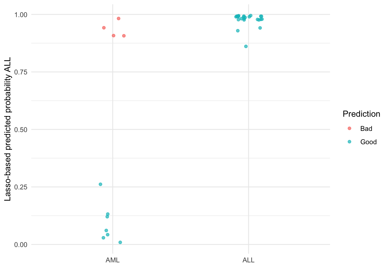
Along with the fact that we reduced the variability of estimation (enough to actually fit a model), introducing bias also helps mitigate over fitting which leads to models that are more generalizable with improved out-of-sample predictions. With this example, we have good (though imperfect) separation between the two subtypes.
This is not the only benefit of introducing bias here. Penalties like the lasso produce sparse fits, with many coefficients set exactly to zero (the second “s” in lasso does literally stand for selection). Weak and noisy predictors are removed, leading to more interpretable glass-box models.
The Pitfall of Debiasing
That being said, it is reasonable to think that reducing the bias of the estimates for \(\boldsymbol{\beta}\) would lead to better predictive performance. One such example is the debiased lasso (also known as the desparsified lasso, Zhang and Zhang (2014)) . However, while this method may be good for providing asymptotically unbiased estimators, debiasing can come at the cost of reintroducing a high amount of variance.
As a result, debiasing often leads to noticeably worse predictions. To see this, we will fit the desparsified lasso to our leukemia dataset.
## Takes about 20 minutes; cached
debiased_fit <- hdi::lasso.proj(Xtrain, ytrain, family = "binomial", lambda = lambda_min)
saveRDS(debiased_fit$bhat, "debiased_fit.rds")
In the code below, we re-estimate the intercept after we obtain the debiased estimates. Then, we can visualize the predictions as we did with the lasso.
debiased_fit <- readRDS("debiased_fit.rds")
debiased_res <- data.frame(
  predicted_prob_ALL = plogis(estimate_intercept(debiased_fit, Xtrain, ytrain) + Xtest %*% debiased_fit),
  class = factor(ytest, levels = c(0, 1), labels = c("AML", "ALL"))
)

debiased_res$prediction_quality <- ifelse(
  debiased_res$predicted_prob_ALL > .5 & debiased_res$class == "AML" |
    debiased_res$predicted_prob_ALL < .5 & debiased_res$class == "ALL",
  "Bad",
  "Good"
)

ggplot(debiased_res, aes(x = class, y = predicted_prob_ALL, color = prediction_quality)) +
  geom_point(alpha = 0.7, position = position_jitter(width = .1)) +
  theme_minimal() +
  scale_color_discrete(name = "Prediction") +
  ylab("Debiased-lasso-based predicted probability ALL") +
  xlab("")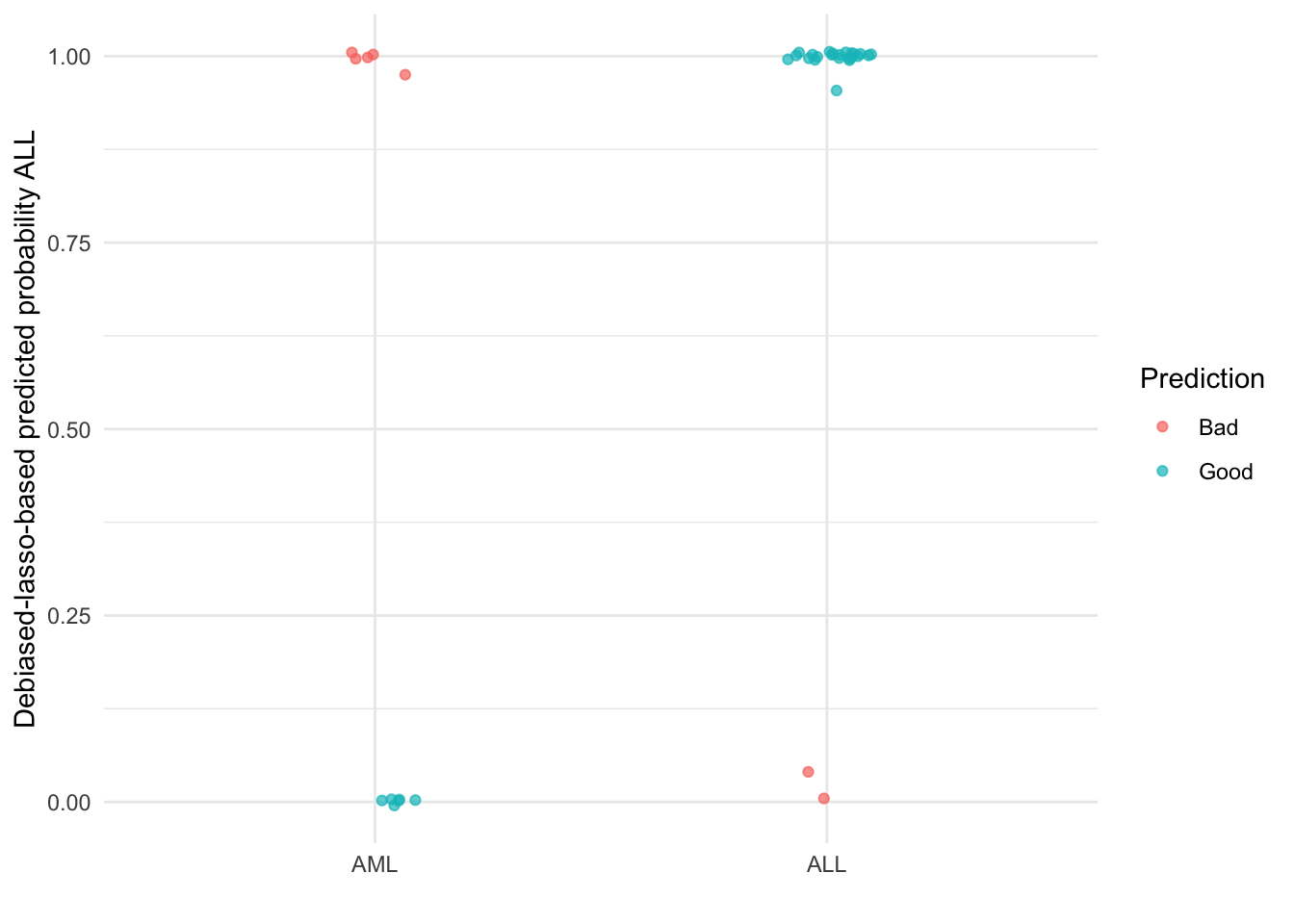
Debiasing the original lasso point estimates results in 1 additional subject with AML being misclassified into the ALL group. Additionally, whereas the lasso correctly predicted all subjects with ALL, debiasing leads to 2 incorrect AML predictions. This is a reduction in accuracy from 87.5% to 78.1%!
While you might say you don’t care about prediction, in a future post we will explore why you can’t afford not to.
Take aways
- Biased estimation can improve a model’s predictive performance
- Reducing bias (via debiasing) often worsens predictions
- The lasso and other penalized regression methods can yield better glass-box models
Follow-up Questions
The following questions might be of interest for new posts:
- What implications does bias have on inference and model interpretation?
- When might debiasing be a good idea?
References
Golub, Todd R., Donna K. Slonim, Pablo Tamayo, Christine Huard, Michael Gaasenbeek, Jill P. Mesirov, Hilary Coller, et al. 1999. “Molecular Classification of Cancer: Class Discovery and Class Prediction by Gene Expression Monitoring.” Science 286 (5439): 531–37. https://doi.org/10.1126/science.286.5439.531.
Zhang, C. H., and S. S. Zhang. 2014. “Confidence Intervals for Low Dimensional Parameters in High Dimensional Linear Models.” Journal of the Royal Statistical Society: Series B (Statistical Methodology) 76 (1): 217–42.
Citation
For attribution, please cite this work as:
Harris, Logan. 2025. “Does Debiasing Estimates Lead to Better
Predictions?” Data Diction (blog). December 15, 2025. https://doi.org/10.59350/h2397-twd61.
